
Allele Based Inference on Evolution and Extinction; A Genetic Drift Approach
Abstract
In other to present a series of stochastic models from population dynamics capable of describing rudimentary aspects of genetic evolution, we studied two-allele Wright–Fisher and the Moran models for evolution of the relative frequencies of two alleles at a diploid locus under random genetic drift in a population of fixed size “simplest form, selection, and random mutation”. Principal results were presented in qualitative terms, illustrated by Monte Carlo simulations from R and http://www.radford.edu/~rsheehy/Gen_flash/popgen. Moran and the Wright-Fisher Models exhibited the same fixation probabilities, only that the Moran model runs twice as fast as the Wright-Fisher Model. A clue that can help us to understand this result is provided by the variance in reproductive success in the two models. Genetic changes due to drift were neither directional nor predictable in any deterministic way. Nonetheless, genetic drift led to evolutionary change in the absence of mutation (P=0.5), natural selection or gene flow. In general, alleles drift to fixation is significantly faster in smaller populations. Probability of fixation of an allele A was approximately equivalent to the initial frequency of that allele. With the inclusion of selection in our model, probability of fixation of a favoured allele due to natural selection increased with increase in fitness advantage and population size. The time taken to reach fixation is much slower, in case of no selective advantage, than a fixation under mutation with selective advantage.
Article Information
- Received
- Accepted
- Published
Academic Editor: Masoud Mohammadnezhad, Associate Professor, Public Health (Health Promotion), School of Public Health & Primary Health Care, Fiji National University, Iran.
Checked for plagiarism: Yes
Review by: Single-blind
Copyright © 2019 S. Oluwafemi Oyamakin, et al.
 This is an open-access article distributed under the terms of the Creative Commons Attribution License, which permits unrestricted use, distribution, and reproduction in any medium, provided the original author and source are credited.
Corresponding author: S. Oluwafemi Oyamakin, Department of Statistics, University of Ibadan, Nigeria —
Competing Interests
The authors have declared that no competing interests exist.
Funding
No specific funding statement was provided by the authors.
Data Availability
No data-availability statement was provided by the authors.
Citation:
Introduction
This paper aim to presents a series of stochastic models from population dynamics capable of describing rudimentary aspects of genetic evolution 11, 12, 13, 14, 15, 16, 17. With focus on the Wright-Fisher model and its variant 5, 6, 7, 8, 9, 10, the Moran model 2; we describe a population of individuals (genes) of different types (alleles) organized into a finite population and where the change in composition of the population is caused by pure genetic drift i.e. randomness with no underlying deterministic behaviour 19. We demonstrate that stochastic computer simulation is an important method for comparing the evolutionary patterns 5, 6 and processes associated with radically different intervals of time.
Methodology
The Wright-Fisher Model
We consider a finite population of 2N genes (or alternatively –N diploid organisms) with each haploid possessing either allele A or allele a, which assumes random reproduction, and generations are not overlapping,
Let xtbe the number of offspring at time t, in the state space 5, 6, 7, 8
S2N = {0,1,…,2N} ……(1)
Let the initial generations contain igenes of allele A and 2N - igenes of type a. Then we define a probability of choosing an A allele for the next generation (success) as:
P = i/2N …..(2)
and the probability of choosing a non-allele A (failure) for each Bernoulli trial as:
P’ = 1 - i /2N ……(3)
Where iis the initial frequency of allele A
Then the transition probabilities from xt to xt+1 is determined by sampling with replacement of 2N independent Bernoulli trials such that xt+1 = j is a binomial random variable from the genes of Generation t. For any integer i, j: X0, …, Xt – 1 in the state space, we have
P(xt+1 = j/Xt= i xt+1 = xt-1 = xt-1 ,…, = X0 = x0) = P(xt+1 = j/Xt= i) ……….(4)
This implies that given the present, the future is conditionally independent on the past. This expression which characterizes the Markov chain in general is the key to analyze the Wright-Fisher model, computed according to the binomial distribution as
P(xt+1 = j/Xt= i =Pij= (2N/j) (i/2N)j (1 –i/2N)2N-j
Pij=(2N/j) pjq2N-j ………(5)
We can use (5) to describe a “transition probability matrix” for the Wright-Fisher model, which gives the probability of going from any state i to any state j in one generation, 1.
We represent the initial state of the system using a vector
ρ(0) = (ρ0(0) ρ1(0) ρ2(0) …)
ρ = (p(X(0) = 0) p(X(0) = 1) p(X(0) = 2)…) …..(6)
This Explains how the Markov Chain Starts
For example, if the population initially had two copies of the allele, then p(X(0) = 2)=1 and all other entries in this vector are zero.


And therefore the transition of the system is then given by the matrix equation;

Each column sums to one because a population that starts with i copies of the allele must have some number between 0 and N copies in the next generation
P t+1 = ρ p t ⇒ ρ = p t+1 / p t ……..(11)
The elements p ij in (10) are called the one step transition probabilities. More generally the n- step transition probability matrix is given by
pij(n) = p(Xn=j/X0 = i …….(12)
By the Chapman Kolmogorov Equation

And by Extension, Markov Probability

The helpful part about writing (10) in matrix form is that it can be iterated using the rules of matrix multiplication
The Moran Model
This model due to 2, although less popular than the WF model amongst biologists, represents a mathematically attractive alternative. This model is also known as a birth-and-death model.
Consider a Moran model for the evolution of a population of size N in which we track the number of individuals with a novel mutant allele (X) versus the number of individuals with the ancestral allele (N-X). Since the population size is a constant, this model has only one independent variable (X). Under the Moran model, evolution occurs when one individual is chosen to reproduce and, simultaneously, one individual is chosen to die.
let X be a random variable, representing the frequency of alleles of type A in the population, to replace individual X, we choose an individual at random from the population (including X itself) to be the parent of the new individual. Thus the model allows only one-step" transitions in which X either decreases or increases, but both transitions occur at the same rate, such that in population t + 1, the number of alleles A can be either (j = i - 1), (j = i + 1), or j = i.
The system can go from i to i+1 if A is chosen to reproduce an offspring and a is chosen to die, expressed as;
Pi,i-1 =(2N-i/2N) .(i/2N)
= (1-p) …….(15)
Where p=i/2N
Similarly, if it is A that is chosen to die and a is chosen to reproduce, then the system can go from ito i-1, expressed below as;
Pi,i+1=(2N-i/2N) .(i/2N)
=p (1 - p) ……(16)
it takes either A to reproduce and die or a to reproduce and die, for the system to go from i to i, expressed as :
Pi,I= (2N-i/2N .(2N-i/2N)+ (i/2N .i/2N)
=p2+ (1-p)2 …….(17)
Where p = i/2N
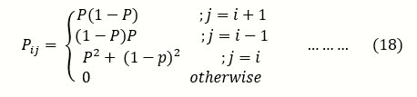
And therefore the transition probability for the implied Markov chain for the Moran model is given by;
The probability of A to reach fixation is called the fixation probability. This holds true, for any neutral model of pure random drift (no mutation and selection) in an unstructured population, at that point, the population is composed of only A genes (Xt= 2N) or a genes (Xt= 0) . That is, with probability one, either of the absorbing states (either 0 or 2N) is eventually entered.
Thus, for 0 < j < 2N,

The probability of extinction given that it started with i copies is;

And the probability of fixation given that it started with i copies is;
Note that with the martingale property (i.e. a random process without bias), the expectation at each time step is expected to be the same;
E(Xt)=E[E(Xt/Xt-1)]=E(Xt-1)=E(Xt-2)
= pA. 2N
= i/2N . 2N
= i …………..(22)
This shows that the expected allele frequency is constant, 3 called this property the constancy of expectation, and nonetheless variability must be lost eventually through chance 4.
Let,
u(i)= P (Xt= 2N/Xt = i) ……..(23)
Be the probability that A is eventually fixed in a population of size 2N that initially contains i copies of A.
then,
i = E[Xt/X0= i] = 2N.P (Xt=2N/X0=i) + 0.P (Xt= 0/X0= i)
i = E [Xt/X0 = i]=2N.P (Xt= 2N/X0 = i)
i = E [Xt/X0= i] = 2N.u(i)
∴i=2N.u(i)
u(i) = i/2N ……..(24)
In an identical manner, we can also express the probability that A eventually becomes lost in the population (extinction at 2N).
Let,

Be the Probability of Extinction
Then,
i = E [Xt/X0 =i] = 0.
P (Xt= 2N/X0 = i) + 2N. P (Xt= 0/X0 = i)
i = E [Xt/X0 = i] = 2N. P (Xt=0/X0 = i)
I = E[Xt/X0=i] = 2N. (1-u(i))
∴i=2N.(1-u(i)
i = 2N-2N. u(i)
∴u(i) = 1– i/2N ……(26)
A similarity between the Moran model and the WF-model is that both models have the same fixation probabilities. The only difference is that the Moran model runs twice as fast as the WF-model, a result we will show in the next chapter.
The Monte Carlo Experiment
The Monte Carlo model 18 simulates genetic drift using a random number generator to sample genes from a small parental population and passes them on to offspring. Population size is assumed to be constant from generation to generation and gene frequency changes the result only from the random sampling process. 2N individuals will be simulated in the population, and in each generation each individual will reproduce randomly and independently 19. This could store the results for each generation in a data frame and then allow one to plot them in a graph.
Experiment 1
Population Size (To investigate the effect of population size and genetic drift)
The population size is allowed to change and to see a graphical display of the change in frequency of allele A overtime in generations, each different line is a separate locus (replicate). Fixation of allele A occurs when its frequency reaches 1.0, which implies extinction of allele a. Running unlinked loci simultaneously (collectively), each with initial gene frequencies of 0.5 is used to explore the effect of changing the population size by running the programme for different population sizes between 5 and 50. Each time we run the simulation, we;
Record the number of fixed loci for A and for a as well as the number of loci which remain polymorphic.
Approximate the number of generations until fixation and extinction for each population explored.
Simulations were repeated 20, 50 and 100 times for a total of 5 replicates for each population size.
Experiment 2: Fixation
To explore the number of generations it takes for one type to either fixes or go extinct, we will run unlinked loci simultaneously (collectively), each with an initial population size of 10, and simulations will be for 100 generations. To explore the fixation of an allele, by running this program for different population sizes, we will record the total number of loci fixed for allele A each time we run the simulation.
Markov Chain Monte Carlo (MCMC) 18, 19, a widely applicable stochastic simulation method. Instead of attempting to minimize the role of chance, MCMC instead introduces chance into problems, event those that are deterministic (such as computing the average of a probability distribution).
Design of the Simulation Procedure
Monte Carlo Experiments were Carried out Based on the Following data Generating Processes
1. individual alleles A and a assumed to follow a binomial distribution with parameters 2N and P (where P is the initial proportion of each allele)
2. Values of N were varied as 5, 10, 20 and 50 to represent small and moderate sample of number of individuals in the population.
3. P is 0.5 if alleles are assumed to be contained in the same proportion at generation 0, and P=0.2 if alleles are assumed to be contained in the same proportion at generation 0
4. j will be generated as the number of copies of allele in the next generation.
For all experiments, iterations were made at 20, 50 and 100 times by the same series of random numbers.
Results and Discussions
Figure 1, Figure 2 showed the graphical representation of the drift of 5 alleles with initial frequency of 0.5 in a typical Wright-Fisher Model which showed genetic divergence as a function of population size. These two Plots demonstrate the graphical representation of drift of 5 alleles with initial frequency 0.5 for N=5 and 50 respectively. Every color represents one allele. In the bigger population there is only one allele fixation that occurs after about 25 generation (X2) and another (X3) at about 90th generation while the other alleles (X1, X4 and X5) did not achieve fixation. On the other hand there were relative large amount of alleles fixations in a short time (5-20 generations) of all the alleles in the small population. In general, alleles drift to fixation in Figure 1 significantly faster in smaller populations.
Figure 2 below illustrated the outcome of five replicates of simulation of the Moran’s model starting with i = 50 copies of type A in a population of size N =5 and 50 respectively. The simulations looked similar to those from the Wright-Fisher model without selection (Figure 1). There are differences; however, the allele frequency only jumped by 1/N in the Moran model, whereas much larger jumps can occur in the Wright-Fisher model.
Figure 1. Genetic drift of the process based on the Wright-Fisher’s model when N=5 left and N=50 right
Download figure
The main qualitative difference, however, is the scale along the x axis. There are only 100 generations represented in Figure 1 of the Wright-Fisher model, but 1,000 birth-death events represented in Figure 2 of the Moran model. One might be tempted to conclude that the Moran model exhibits less drift, but this is not a fair comparison. One time step in the Wright-Fisher model involves N births followed by the death of all N parents and so is more equivalent to N birth-death events in the Moran model. Thus, these figures all represent the same total number of generations (100). Over this period, and with only five replicates each, it is unclear which model exhibits more drift. The above results showed that polymorphism lost significantly faster in the Moran model than in the Wright-Fisher model. This seems counter intuitive, because the Moran model makes only little jumps in frequency, whereas the Wright-Fisher model could make large jumps. A clue that can help us to understand this result is provided by the variance in reproductive success in the two models. When reproductive success has more variable, stochasticity (here, random genetic drift) plays a stronger role, and polymorphism will be lost by chance more rapidly.
For our genetic model, we can also describe Figure 2 with a “transition probability matrix” for the Wright-Fisher model, which gives the probability of going from any state ito any state j in one generation. Because we could have anywhere from 0, 1, 2, to N copies of type A, this matrix has N +1 rows and columns, in our population of size five, the transition probability matrix isto j from i

Each rows sum to one because a population that starts with icopies of the allele must have some number between 0 and 2N copies in the next generation:

The first and last rows are particularly simple because there is no mutation; if nobody is type A (i= 0; first column) or if everybody is type A (i= N; last column), then no further changes are possible.
The matrix pij can be iterated using the rules of matrix multiplication. P2tells us the probability that there were j copies at time t+2 given that there was icopies at time t. In general, Pt tells us the probability that there were j copies at time t given that there was icopies at time 0. For example, calculating P100 using equation (using a mathematical software package) gives

(The zeros in the middle of this matrix are not exactly zero, but they are less than 10_156).
The initial state of the system is represented using a vector, since our population initially had two copies of the allele, then P(X (0) =2) =1 and all other entries in this vector are zero.
ρ(0) = (0 0 1 0 0 0)
Multiplying P100 on the right by this initial vector, gives;

The vector on the right indicated that there is approximately 50% chance that type A will be lost (j =0) after 100 generations and a 50% chance that type A will be fixed (j=5).
These results suggested that if we start with icopies of type A, then type A will eventually be lost with probability 1-i/2N and fixed with probability i/2N
Given that no clear conclusions emerge from a few replicate simulations, we must run many more replicate simulations to compare the Wright-Fisher and Moran models. Starting with p (0) = 0.5 and p (0) = 0.2 in a population of size from 5 to 50, we ran 20, 50 and replicate simulations on each population until fixation or loss of type A.
Table 1 showed the simulation results for the Wright-Fisher model at different population sizes (N=5, 10, 20 and 50) and replicate simulations of (20, 50 and 100) contained at the same proportion at 0.5 and 0.10 which is in parenthesis. For the Wright-Fisher Model and the Moran Model, at a population size of 5 and at the various iterative levels, the probabilities of fixation are 0.6, 0.52, 0.57 and 0.45, 0.44, 0.51 respectively. Also at a population size of 10 and at the various iterative levels, the probabilities of fixation are 0.55, 0.52, 0.51 and 0.40, 0.56, 0.59 respectively. For p (0) = 0.2, the Wright-Fisher Model and the Moran Model, at a population size of 5 and at the various iterative levels, the probabilities of fixation are 0.25, 0.22, 0.23 and 0.15, 0.15, and 0.06 respectively. Also at a population size of 10 and at the various iterative levels, the probabilities of fixation are 0.25, 0.26, 0.24 and 0.40, 0.56, 0.59 respectively. This result showed that the probability of fixation of an allele A is approximately equivalent to the initial (starting) frequency of that allele. The result in the table above showed that assuming genetic drift is the only evolutionary force acting on an allele, at any given time the probability that an allele will eventually become fixed in the population is simply its frequency in the population at that time i.e. probability of an allele fixing is almost the same as the starting frequency.
Table 1. Probabilities of fixation of the allele A at P=0.5 and P=0.2 in parenthesis| WRIGHT-FISHER MODEL | MORAN MODEL | |||||||
| N=5 | N=10 | N=20 | N=50 | N=5 | N=10 | N=20 | N=50 | |
| 20 | 0.6(0.25) | 0.55(0.25) | 0.50(0.10) | 0.15(0.15) | 0.45(0.25) | 0.40(0.25) | 0.6(0.15) | 0.60(0.15) |
| 50 | 0.52(0.22) | 0.52(0.26) | 0.46(0.15) | 0.15(0.15) | 0.44(0.24) | 0.56(0.26) | 0.44(0.30) | 0.50(0.24) |
| 100 | 0.57(0.23) | 0.51(0.24) | 0.38(0.24) | 0.06(0.06) | 0.51(0.23) | 0.59(0.23) | 0.39(0.23) | 0.43(0.20) |
Table 2 showed the comparison between Wright-Fisher model and the Moran model at different population sizes and the variance of reproductive individuals. This table revealed that Moran Model exhibits twice the variance in reproductive success and therefore consequently, this indicated more genetic drift towards Wright Fisher Model. In the Wright-Fisher model, the variance in reproductive success of single individuals, r 2, is given by the binomial variance N p (1 =p) from equation (5). When there is a single individual (i.e., with p =1/N). Thus, r =1-1>N. To calculate the variance in reproductive success over a single birth-death event in the Moran model, we use the formula for calculating variance, summing the squared change in number of copies over all possible transitions using equation (18). Since the time to fixation varies between simulations, to obtain a sense of the possibilities, we simulated the fate of our population of alleles large number of times, until fixation and extinction are achieved, We then summarize the distribution by finding the mean fixation time and average extinction time.
Table 2. Variance of Reproductive Success| WRIGHT FISHER MODEL | MORAN MODEL | |
| N=5 | 1.25 | 2.5 |
| N=10 | 2.5 | 5.0 |
| N=20 | 5.0 | 12.5 |
| N=50 | 12.5 | 25.0 |
At different number of iterations and population sizes, table 3 showed the average time until fixations and extinctions in the Wright-Fisher Model and Moran Model in parenthesis.
Table 3. Average Time until Fixation and Extinction of the allele A in the Wright-Fisher Model and Moran Model in parenthesis.| N=5 | N=10 | N=20 | N=50 | |||||
| Average time until fixation | Average time until extinction | Average time until fixation | Averagetime until extinction | Average time until fixation | Average time until extinction | Average time until fixation | Averagetime until extinction | |
| iterations | ||||||||
| 20 | 8.20(13.0) | 11.50 (11.1) | 24.80(14.22) | 21.11(46.25) | 47.70(40.33) | 42.75(56.38) | 64.5(140.92) | 74.00(136.50) |
| 50 | 13.92 (13.5) | 10.0(11.96) | 25.15(27) | 25.04(22.77) | 50.39(49.59) | 43.71(47.14) | 68.89(151.08) | 71.17(147.72) |
| 100 | 15.07(13.57) | 9.8(12.43) | 23.53(25.46) | 24.71(26.83) | 48.76(52.38) | 40.38(49.48) | 65.33(122.65) | 65.35(110.90) |
| Average | 12.40(13.51) | 10.47(11.83) | 36.74(33.57) | 23.62(31.95) | 48.95(47.43) | 42.28(51.12) | 66.24(138.22) | 70.35(131.71) |
We can see from the table that the time to fixation or extinction of an allele is related to population size. The larger the population size, the longer it takes to achieve fixation, i.e. Probability of fixation is also influenced by population size for both Models
Our models allow the inclusion of other evolutionary forces: selection and mutation
Selection
So far, we have considered only neutral models of evolution, that is, those for which there is no preference for a particular allele. Despite being apparently a reasonable model for some aspects of genetic, ecological or linguistic behavior, geneticists in particular have been interested in the fate of alleles that are selected for or against 20. The relationship between the genetic make-up of an individual and its survival is of course very complicated. However, one can explore the effects of selection by simply introducing parameters that determine how many offspring an individual carrying a particular allele (or combination of alleles when diploid organisms are being considered) has on average. In this section we offer a small taste of some evolutionary models that encompasses selection. Fitness here is a measure of reproduction and survival.
AA=1.0, Aa=0.75 and aa=0.50
Here, the allele A is more fit than the type a and began at a frequency of p (0) =0.2. The simulations were run for populations of sizes N = 5, 10, 20 and 50. In all cases, the alleles rose in frequency towards fixation within 100 generations. When the population size was small, the Wright-Fisher model exhibits more variability around the deterministic trajectory than when the population size was large. When N was only 5 and 10, we observed extinction of the beneficial allele in one of the five replicates, which made the probability of fixation to be 0.95 and 0.9 respectively, however, when population size became larger (N=20 and 50), none of the replicates went into extinction, and had the probability of fixation to be 1.0. Similar behavior occurred at a frequency of p (0) =0.5. Irrespective of the population size, there was not an extinction of the beneficial allele in any of the five replicates, which gave the probability of fixation to be 1.0. The probability of fixation of a favored allele due to natural selection increases with increased fitness advantage and with increased population size.
Also, in table 4, results showed that selection alone drives the system into a state consisting of only the better fit variant thereby prevented the detrimental allele from increasing in the population.
Table 4. Probabilities of Fixation and Average Time until Fixation of the allele A with Selective Advantage at P=0.2 and P=0.5 in parenthesis.| Probability of fixation | Average time until fixation | |
| N=5 | 1.0 (0.95) | 6.6(11.42) |
| N=10 | 1.0 (0.90) | 14.0(13.94) |
| N=20 | 1.0 (0.10) | 11.5(15.50) |
| N=50 | 1.0 (0.10) | 15.35(19.00) |
These figures illustrated an important point: adding stochasticity to a model need not cause major changes to the results. In populations of small size (N = 50), we have seen allele frequency changed when there should have been none (the neutral case, Figure 2), and we have witnessed the loss of a beneficial allele, which we would expect to fix (table 4). We observed that when the amount of chance (here represented by variation in samples from the binomial distribution) is small relative to other forces like selection, stochastic models can behave very much like deterministic models.
Figure 2. Genetic drift of the process based on the Moran’s model when N=5 and N=50
Download figure
Over Dominance (Aa has the Highest Fitness)
Over dominance = heterozygote most fit. Surprising things happen when the heterozygote is most fit.
In table 5, alleles initial frequencies were not 50/50, Strong selection was acting, but the allele frequencies did not change (compared with table 4). At a population size of 5, the probability of fixation was 0.95, at a population size of 10, the probability of fixation was 0.9 but at population size of 20 and 50 respectively, there was no fixation of any of the alleles. This was because genetic drift was a function of population size. The population was said to be at equilibrium state. The ratio 50/50 was because the homozygotes are equally bad. In table 5, the A allele begins at a frequency of p (0) =0.5, simulations were ran for populations of sizes N = 5, 10, 20 and 50. In all cases, the alleles increased in frequency towards fixation within 100 generations.
Table 5. Probabilities of Fixation and Average Time until Fixation of the A allele with Over Dominance at P=0.2 and P=0.5 in parenthesis| Probability of fixation | Average time until fixation | |
| N=5 | 0.95 (1.0) | 39.0 (25.60) |
| N=10 | 0.6 (0.8) | 45.33 (38.25) |
| N=20 | 0.0 (0.6) | - (44.33) |
| N=50 | 0.0 (0.0) | - (-) |
At a population size of 5, all alleles experienced fixation (probability of fixation =1.0). At a population size of 20. However, not all alleles experienced fixation (probability of fixation = 0.6), but a population size of 50, no allele experienced fixation (probability of fixation =0). The larger the population size, the longer it takes to achieve fixation.
Example of heterozygote most fit is the case of the sickle-cell trait (in the presence of malaria)
A/A people die of malaria
S/S people die of sickle-cell anemia.
In conclusion, table 5 showed that over dominance maintain allele at high frequency in a population and guaranteed the stability of genetic polymorphism.
Under Dominance (Aa has the Lowest Fitness)
Under dominance= heterozygote less fit
Here alleles are not contained in the same frequency in generation 0. At a population size of 5, probability of fixation = 0.25, at a population size of 20 however, probability of fixation reduced to 0.1, but a population size of 50, no allele experienced fixation (probability of fixation =0), all these indicated high probability of extinction (fixation of the allele a). Allele a will fix even though it does not maximizes population fitness. The population rolls to a small fitness peak, even though a larger one is possible. Population, which is fixed for allele a will, resists introduction of allele A. Here alleles are contained in the same frequency in generation 0, equilibrium is said to exit and the population is unstable. At a population size of 5, probability of fixation = 0.9, at a population size of 20, probability of fixation reduced to 0.9, but a population size of 50, all the alleles experienced fixation (probability of fixation =1.0), all this indicates high probability of extinction of the a allele. Table 6
When the heterozygote has the lowest fitness, the system is considered unstable, allele frequency will move until either A or a is fixed. Equilibrium occurs at 50% of each allele.
When P (A) is above equilibrium A will be fixed.
When P (A) is below equilibrium a will be fixed.
Example of the under dominance is the African butterfly pseudacraea eurytus, the orange and blue homozygotes each resemble a local toxic species, but the heterozygote resembles nothing in particular and is attractive to predators.
Although mutation is sometimes considered as the raw material of evolution, it is a very weak force in changing allele frequency. As shown in table 12 above, starting with an initial frequency of 0.2, it will take a hundred generations to change the frequency of the A allele to 0.1998 and a thousand generations to change the frequency to 0.198. Suppose alleles are contained in the same proportion with a frequency of 0.5, after a hundred generations, the frequency of the A allele will change 0.499 and a thousand generations to change the frequency to 0.495. But suppose only A alleles are contained in the population with a frequency of 1.0, after a hundred generations, the frequency of the A allele will change to 0.998 and a thousand generations to change the frequency to 0.990. Table 7
In table 8, the A allele begins at a frequency of p (0) =0.2 and p (0) =0.5. At a population size of 5, the probability of fixation was 0.15 with an average time until fixation to be 16.00, when the population size became 10, the probability of fixation was 0.2 with an average time until fixation of 29.6, but when the population size became 20, the probability of fixation was 0.25 with an average time until fixation of 60.0. The larger the population size, the longer it takes to achieve fixation. These results indicated that the probability of fixation with or without mutation rate was still approximately its initial frequency.
Table 6. Probabilities of Fixation and Average Time until Fixation of the A allele with Under Dominance at P=0.2 and P=0.5 in parenthesis| Probability of fixation | Average time until fixation | |
| N=5 | 0.25 (0.9) | 10.8 (5.94) |
| N=10 | 0.1 (0.95) | 9.5 (7.84) |
| N=20 | 0.1 (0.9) | 17.0 (9.67) |
| N=50 | - (1.0) | - (20.0) |
| Numbers of generations | 100 | 200 | 500 | 1000 |
| P=0.2 | 0.1998 | 0.1996 | 0.199 | 0.198 |
| P=0.5 | 0.499 | 0.499 | 0.497 | 0.495 |
| P=1.0 | 0.9990 | 0.998 | 0.995 | 0.990 |
| Probability of fixation | Average time until fixation | |
| N=5 | 0.15 (0.45) | 16 (7.67) |
| N=10 | 0.2 (0.4) | 29.6 (17.7) |
| N=20 | 0.25 (0.2) | 60.0 (43.7) |
| N=50 | - (0.1) | - (64.75) |
At a population size of 5, the probability of fixation was 0.45 with an average time until fixation to be 7.67, when the population size became 10, the probability of fixation was 0.4 with an average time until fixation of 17.7, but when the population size became 20, the probability of fixation was 0.2 with an average time until fixation of 43.7. The larger the population size, the longer it takes to achieve fixation.
These results indicated that the probability of fixation with or without mutation rate was still approximately its initial frequency.
In table 9, the A allele begins at a frequency of p (0) =0.2. at a population size 5, the probability of fixation is 0.8 while the average time until fixation was 9.38,but at a population size of 10, 20 and 50, the probability of fixation was 1.0 while the average time until fixation were 13.65, 15.95 and 19.50. This indicated that the larger the population, the longer it takes to achieve fixation.
In table 9, the A allele were assumed to be at a frequency of p (0) =0.5 in the first generation. Here, irrespective of the population size, all alleles in the five replicates experienced fixation and the average time until fixation for each population was 8.15, 10.22, 9.6 and 13.7. The results obtained in table 9 can be compared to table 4. It was noticed that similar results were obtained; this established the fact that mutation alone is a weak force of allelic evolution.
Table 9. Probabilities of Fixation and Time until Fixation of the A allele with Selective Advantage and Mutation Rate (µ= 1 * 10-5, v= 1* 10-6) at P=0.2 and P=0.5 in parenthesis| Probability of fixation | Average time until fixation | |
| N=5 | 0.8 (1.0) | 9.38 (8.15) |
| N=10 | 1.0 (1.0) | 13.65 (10.22) |
| N=20 | 1.0 (1.0) | 15.95 (9.6) |
| N=50 | 1.0 (1.0) | 19.50 (13.7) |
There is a behavioural difference between mutation with and without Selective Advantage. The time taken to reach fixation is much slower, in case of no selective advantage, than a fixation under mutation with selective advantage. To illustrate the difference between the two types of mutation, from the results obtained in table 8, table 9 above, a population size of 5 individuals and with a life time of 100 years. Under these conditions, it will take a neutral mutation, on average 16 years to become fixed in the population, but when we compared to a mutation with selective advantage(s) of 0.00001, the mutation will become fixed in the same population in only 9.38 years. If the selection coefficient is much larger than the mutation rate, there exists a broad interval of population sizes, in which weakly diverse populations are almost neutral while highly diverse populations are controlled by selection pressure.
Conclusions and Recommendation
The procedure of stochastic modeling is not, of course, restricted to statistics. In particular, stochastic models have played a pivotal role in understanding the dynamics of evolutionary systems and as such one sees many similarities in the approaches and methods that have been used to those employed by Statistician. This paper has been a review of the ideas and formalism used to model stochastic processes in fields that statistical physicists are not typically acquainted with, specifically population genetics, ecology and linguistics. As a consequence, some parts of the discussion will seem familiar, other parts will not. We have tried, and we hope that we have succeeded, to explain the background ideas and motivation, since this will be the greatest obstacle to understanding among a readership of statistical physicists. On the other hand the degree of mathematical sophistication that has been assumed is greater than would be typical outside physics or mathematical biology.
In our discussions of the mathematical models, we have mostly used the language of population genetics, but the results obtained are more widely relevant. As the evolutionary paradigm becomes even more widely applied, there may be other areas in which analogies can be drawn. It is interesting to know how neutral processes turned out to have greater importance in all three areas we discussed. At the very least, neutral theories can be thought of as null models, against which data and other models can be compared. Most textbooks in population genetics begin their discussion of genetic drift with the Wright–Fisher model, although for physicists the use of non-overlapping generations and a ‘time’ measured in number of generations will not appear so natural. The Moran model, which has exactly the same limit when the number of genes becomes large, is far more familiar, resembling a birth/death process where a death is immediately followed by a birth. In addition, the continuous time limit may easily be taken, leading to a master equation of a kind well known in statistical physics.
In genetics, ecology or language, just as in physics, reality cannot be described by ideal models; there will be a multitude of ways in which real systems deviate from the ideal models created by scientists when they first enter a field. One of the methods that have been devised by population geneticists to deal with this will be very familiar to physicists. This is to characterize a non-ideal system by a few parameters, which will hopefully, if chosen correctly, capture the essence of the system. It may be that a simple model can then be utilized, but with these parameters built in. An example is the effective population size, N, discussed in the literature, which reflected how the non-ideal nature of the system changes the effective value of N: the effective size of the real population being the number of individuals in the ideal population which gave the same magnitude for the quantity of interest. The reason of our interest is not just the mathematical elegance of these models, but with the availability of massive amount of sequencing data. We actually can use these models (or advanced models incorporating variable population size, mutation effect etc., to solve and answer real questions in molecular biology. The stochastic evolution of a DNA segment that experiences recombination is a complex process; so many analyses are based on simulations. The aim of this paper is to give an account of useful analytical results in population genetics, together with their proofs.
References
- 1.S P Otto, Troy Day. (2007) . A Biologist’s Guide to Mathematical Modeling in Ecology and Evolution.PrincetonUniversityPress 744.
- 2.Moran P A P. (1958) Random processes in genetics". Mathematical Proceedings of the Cambridge Philosophical Society 54(1), 60-71.
- 3.Mishra Bud. (1998) Computational Systems Biology: Room 1002, 715 Broadway, Courant Institute. , NYU, New York, USA, Human Population Genomics. Lecture 10.
- 4.F D Hollander. Mathematical Institute, Leiden University, P.O (2013) stochastic models for genetic evolution. , Box 9512, 2300 RA Leiden, The Netherlands. Email:[email protected]
- 5.Carsouw M F J. DenHollander Mathematical Institute, Leiden University (2012) Wright-Fisher evolution Bachelor thesis. 1, Supervisor: Prof. Dr. W.Th.F
- 6.J F Crow. (2010) Wright and Fisher on Inbreeding and Random Drift". Genetics. ISSN 0016-6731. PMC 2845331 , Bethesda, MD:, Genetics Society of America 184(3), 609-611.
- 7.Hailong C, Wangshu Z. (2014) Population Genetics: Wright Fisher Model and Coalescent Process. A Final Project Report Presented in Partial Fulfillment of the requirements for Math 505b.
- 9.R A Fisher. (1930) The Genetical Theory of Natural Selection: a Complete Variorum Edition.OxfordUniversityPress.
- 11.WGBH Educational Foundation; Clear Blue Sky Productions, Inc (2001) Evolution Library (Web resource). "Genetic Drift and the Founder Effect" Evolution. , Boston, MA:
- 12.Freeman S, J C Herron. (2007) . Evolutionary Analysis (4th ed.). Upper Saddle River,NJ:PearsonPrenticeHall .
- 13.Futuyma D. (1998) . Evolutionary Biology (3rd ed.). Glossary p. 300. Sunderland, MA: Sinauer Associates. ISBN 0-87893-189-9. LCCN 97037947. OCLC .
- 15.J D Futuyma. (2009) Natural Selection: How Evolution Works". Action bioscience. Washington, D.C.:American Institute of Biological Sciences.Retrieved2009-11-24.An interview with See answer to question: Is natural selection the only mechanism of evolution?.
- 16.Iwasa Y, Michor F, M A Nowak. (2003) Evolutionary dynamics of escape from biomedical intervention. Proceedings of the Royal Society of London. Series B: Biological Sciences 270 2573.
- 17.Iwasa Y, Michor F, M A Nowak. (2004) Stochastic tunnels in evolutionary dynamics. , Genetics 166, 1571-9.